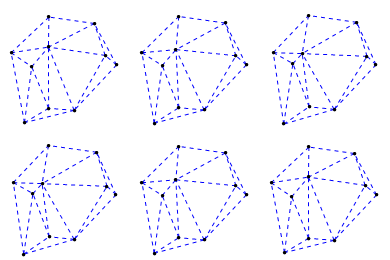
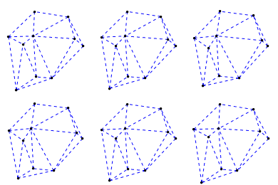
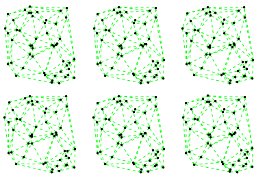
Small Oscillations in a Delaunay Mesh
(You can see more of the images at this page, or a more complete list of images in the the /img/ directory.)
This is a fun exercise in linearizing systems. Physicists like nothing more than making approximations (no, the period of a pendulum is not $2 \pi\sqrt{\frac{\ell}{g}}$). After wasting time on one-too-many (or 30-too-many) classical mechanics class linearization problems I decided to write a program to do it for me in the case of a net of springs. The results are fun, and I provide my mathematica source code.


Now here’s a question: Why does a net of springs in 2D need linearization in the first place? Aren’t springs linear? (Hint: In this simulation the spring potential $V(x,y)$ has a local maximum $V(0,0)$, a global minimum on the circle $x^2+y^2=\ell^2$ with $\ell$ being the resting length of the spring, and goes to infinity as $x,y\to\infty$.)
Mathematica source:
<< ComputationalGeometry`
pts=Join[RandomReal[{-1,1},{45,2}]^3-0.4,RandomReal[{-1,1},{45,2}]^3+0.4];
pts=RandomReal[{-1,1},{50,2}];
edges=Union[Union/@Flatten[(Function[y,{#1,y}]/@#2)&@@@DelaunayTriangulation[pts],1]];
springk=1&/@edges;
masses=1&/@pts;
kmat=SparseArray[Join[edges,(Reverse/@edges )]->Join[springk,springk]];
normalized[v_]:=If[v.v>0,v/Sqrt[v.v],v];
indices=Union[Flatten[edges]];
normals=Table[normalized[pts[[i]]-pts[[j]]],{j,1,Length[indices]},{i,1,Length[indices]}];

(* After linearization, you find that, if kmat[i,j] is the spring constant between points
i and j and "normals" is pts[[i]]-pts[[j]] normalized and {a[i,1],a[i,2]} is the magnitude of the
 small oscillations, the force on a point i due to all the other springs j is: Sum[-kmat[i,j]
  normals[i,j] normals[i,j].({a[i,1],a[i,2]}-{a[j,1],a[j,2]}),{j,1,3}] *)
system=Chop@ Eigensystem[(SparseArray[Flatten[Table[{ {2i+s-2,2j+l-2}->kmat[[i,j]]
normals[[i,j,l]]normals[[i,j,s]]},{j,1,Length[indices]},{l,1,2},{i,1,Length[indices]},{s,1,2}]]]-
SparseArray[Flatten[Table[{2i+s-2,2i+l-2}->Sum[kmat[[i,j]]normals[[i,j,l]]
normals[[i,j,s]],{j,1,Length[indices]}],{i,1,Length[indices]},{s,1,2},{l,1,2}]]]
)];
system={Sqrt[-#[[1]]],Partition[#[[2]],2]}&/@Transpose[system[[All,;;-4]]];

pt2[n_,t_,i_]:=pts[[n]]+0.1system[[i,2,n]]Cos[system[[i,1]]t];
plotme[t_,i_]:=Graphics[{ Green,Thin,Dashed,Line[{pt2[#1,t,i],pt2[#2,t,i]}&@@@edges],Black,Table[Disk[pt2[j,t,i],0.03],{j,1,Length[pts]}]},PlotRange->{ {-1.1,1.1},{-1.1,1.1}}];

(* After running the above functions, call plotme[t,i] for time t and mode i. Make sure 1<=i<=Length[system]. *)